


Portfoliotheorie (portfolio theory)
eröffnet am 10.04.23 20:50:00 von
neuester Beitrag 09.02.24 00:10:12 von
neuester Beitrag 09.02.24 00:10:12 von
Beiträge: 95
ID: 1.368.155
ID: 1.368.155
Aufrufe heute: 3
Gesamt: 2.458
Gesamt: 2.458
Aktive User: 0
Top-Diskussionen
| Titel | letzter Beitrag | Aufrufe |
|---|---|---|
| vor 6 Minuten | 9713 | |
| heute 17:20 | 7219 | |
| vor 2 Minuten | 6227 | |
| vor 28 Minuten | 3487 | |
| vor 15 Minuten | 3419 | |
| heute 09:20 | 2592 | |
| vor 14 Minuten | 2497 | |
| heute 19:52 | 2025 |
Meistdiskutierte Wertpapiere
| Platz | vorher | Wertpapier | Kurs | Perf. % | Anzahl | ||
|---|---|---|---|---|---|---|---|
| 1. | 1. | 17.978,00 | +0,44 | 206 | |||
| 2. | 2. | 168,79 | -0,85 | 103 | |||
| 3. | 3. | 8,6400 | +4,22 | 84 | |||
| 4. | 14. | 0,0164 | +0,61 | 73 | |||
| 5. | 4. | 3,8775 | +5,01 | 62 | |||
| 6. | 11. | 2.302,40 | +0,73 | 42 | |||
| 7. | 9. | 1,0000 | +3,63 | 41 | |||
| 8. | 6. | 6,7280 | +0,81 | 39 |
Beitrag zu dieser Diskussion schreiben
Antwort auf Beitrag Nr.: 75.124.866 von faultcode am 18.01.24 14:39:34
kurz zu Fixed weights (FW):
aus:
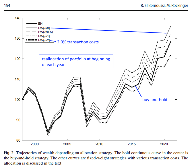
2022, "Rebalancing with transaction costs: theory, simulations, and actual data", Bernoussi, Rockinger (aus der Schweiz)
https://link.springer.com/article/10.1007/s11408-022-00419-6
BH = buy-and-hold strategy
SR = Sharpe Ratio
...
A common practice to counter these changes is called portfolio rebalancing, also known as a fixed-weight strategy (FW). It is a contrarian strategy consisting of selling successful assets and buying losers, thereby restoring a predetermined set of portfolio weights. The main objective of rebalancing is to maintain a given (strategic) asset allocation and therefore maintain the risk profile of the portfolio in line with the risk tolerance of the investor.
...
In practice small pension funds must by law choose long-term portfolio allocations where the weights allocated to different asset categories are given. Similarly for the amount of foreign currency exposure. Large pension funds may decide on broader asset categories and will still give themselves strategic allocations determined by ‘experts’ instead of relying on quantitative models.
...
4 Actual allocation
In this section, we discuss the results of an actual allocation representative of some Swiss pension funds. The pension fund manager has a relatively large set of instruments in which she can invest. Those instruments are a set of well-known stock indices that could be cheaply duplicated by ETFs. Then there are commodities and real estate as alternative assets. On the fixed income side, the manager may invest in short-term interest rates or in 10-year Swiss and 10-year German Government bonds.
...
It turns out that for actual assets, in the long run, the dynamic is sufficiently complex that the given BH strategy is dominated by a fixed-weight strategy as long as transaction costs are relatively small.
...
We notice that it is only with a relatively high transaction cost of 2% for each asset that the fixed-weight strategy no longer dominates the buy-and-hold strategy. In practice, the level of transaction cost is in the range of 0.5%, and therefore, a fixed-weight strategy is interesting.
...
...
From a purely statistical point of view, it turns out that the null hypothesis of the SR of BH being equal to the SR of FW cannot be rejected in the long-run.
...
This table (Table 9/FC) confirms that for all possible allocations, as long as the transaction cost remains below 1%, the SR of the FW allocation is larger than the one for the BH strategy.
...
First, our paper demonstrates that a rebalancing strategy may be advocated for risk-averse investors because it reduces volatility in situations often encountered. This finding corroborates past studies.
The main finding is the relevance of autocorrelation for an asset as well as pairwise correlation among assets.We observe that for a strong mean reversion of assets, the fixed-weight strategy dominates the buy-and-hold one. Concerning pairwise correlation, we show that when assets are negatively correlated, the transaction costs are the highest, and the buy-and-hold strategy is significantly better (except when the market exhibits strong mean reversion). Generally, if a portfolio manager managing a well-diversified portfolio faces transaction costs of less than 2% and if she anticipates a futuremarket with mean reversion, then she should rebalance her portfolio.
...
Finally, even though this is not at the center of our research, we would like to note that rebalancing strategies, because of their deterministic character, exclude any emotions and subjective influences on buying and selling decisions and thus tend to limit behavioral biases.
___
Table 9 ist das Herzstück hier; etwa schwierig zu lesen, da Zwischensummen innerhalb eines Portfolios (gleich eine Spalte) zu beachten sind: Total stocks + Total bonds + Total alternative + Total liquidity = 100%
___
FW scheint dann besser als BH zu funktionieren, wenn man langfristig von Mean reversion (Reversion to mean) bei einer gewählten Asset-Klasse ausgeht und die Transaktionsgebühren beim Rebalancing nicht zu hoch sind.
Allerdings wird hier - für den Privatmensch ja nicht unrelevant mMn - das Thema Steuern (bei Verkauf) nicht erwähnt.
Zitat von faultcode: ...
• (FW: fixed weights ?)
...
kurz zu Fixed weights (FW):
aus:
2022, "Rebalancing with transaction costs: theory, simulations, and actual data", Bernoussi, Rockinger (aus der Schweiz)
https://link.springer.com/article/10.1007/s11408-022-00419-6
BH = buy-and-hold strategy
SR = Sharpe Ratio
...
A common practice to counter these changes is called portfolio rebalancing, also known as a fixed-weight strategy (FW). It is a contrarian strategy consisting of selling successful assets and buying losers, thereby restoring a predetermined set of portfolio weights. The main objective of rebalancing is to maintain a given (strategic) asset allocation and therefore maintain the risk profile of the portfolio in line with the risk tolerance of the investor.
...
In practice small pension funds must by law choose long-term portfolio allocations where the weights allocated to different asset categories are given. Similarly for the amount of foreign currency exposure. Large pension funds may decide on broader asset categories and will still give themselves strategic allocations determined by ‘experts’ instead of relying on quantitative models.
...
4 Actual allocation
In this section, we discuss the results of an actual allocation representative of some Swiss pension funds. The pension fund manager has a relatively large set of instruments in which she can invest. Those instruments are a set of well-known stock indices that could be cheaply duplicated by ETFs. Then there are commodities and real estate as alternative assets. On the fixed income side, the manager may invest in short-term interest rates or in 10-year Swiss and 10-year German Government bonds.
...
It turns out that for actual assets, in the long run, the dynamic is sufficiently complex that the given BH strategy is dominated by a fixed-weight strategy as long as transaction costs are relatively small.
...
We notice that it is only with a relatively high transaction cost of 2% for each asset that the fixed-weight strategy no longer dominates the buy-and-hold strategy. In practice, the level of transaction cost is in the range of 0.5%, and therefore, a fixed-weight strategy is interesting.
...

...
From a purely statistical point of view, it turns out that the null hypothesis of the SR of BH being equal to the SR of FW cannot be rejected in the long-run.
...
This table (Table 9/FC) confirms that for all possible allocations, as long as the transaction cost remains below 1%, the SR of the FW allocation is larger than the one for the BH strategy.
...
First, our paper demonstrates that a rebalancing strategy may be advocated for risk-averse investors because it reduces volatility in situations often encountered. This finding corroborates past studies.
The main finding is the relevance of autocorrelation for an asset as well as pairwise correlation among assets.We observe that for a strong mean reversion of assets, the fixed-weight strategy dominates the buy-and-hold one. Concerning pairwise correlation, we show that when assets are negatively correlated, the transaction costs are the highest, and the buy-and-hold strategy is significantly better (except when the market exhibits strong mean reversion). Generally, if a portfolio manager managing a well-diversified portfolio faces transaction costs of less than 2% and if she anticipates a futuremarket with mean reversion, then she should rebalance her portfolio.
...
Finally, even though this is not at the center of our research, we would like to note that rebalancing strategies, because of their deterministic character, exclude any emotions and subjective influences on buying and selling decisions and thus tend to limit behavioral biases.
___
Table 9 ist das Herzstück hier; etwa schwierig zu lesen, da Zwischensummen innerhalb eines Portfolios (gleich eine Spalte) zu beachten sind: Total stocks + Total bonds + Total alternative + Total liquidity = 100%
___
FW scheint dann besser als BH zu funktionieren, wenn man langfristig von Mean reversion (Reversion to mean) bei einer gewählten Asset-Klasse ausgeht und die Transaktionsgebühren beim Rebalancing nicht zu hoch sind.
Allerdings wird hier - für den Privatmensch ja nicht unrelevant mMn - das Thema Steuern (bei Verkauf) nicht erwähnt.
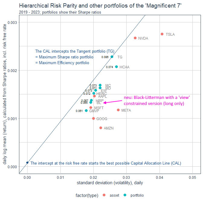
Antwort auf Beitrag Nr.: 75.140.689 von faultcode am 21.01.24 22:32:22Update Vola-Rendite-Diagramm mit obigem Black-Litterman-Portfolio (BL):

Antwort auf Beitrag Nr.: 75.216.851 von faultcode am 04.02.24 19:46:44
--> es war Michael Hartnett, Bank of America's chief investment strategist, ab Mai 2023: https://www.npr.org/2023/12/13/1216457187/wall-street-magnif…
In May, a few months after OpenAI debuted its ChatGPT tool, Hartnett noticed investors were channeling their enthusiasm for artificial intelligence into a small basket of established tech companies.
Mittlerweile sind es aber nur noch die "Fab Five":
January 30, 2024
https://finance.yahoo.com/video/magnificent-seven-stocks-now…
--> Nvidia, Meta Platforms, Google, Microsoft und Amazon
=> nach geschätzt 8 Monaten sind also so gesehen zwei Plätze frei geworden in den Magnificent 7: damit komme ich auf einen Turnover (nicht annualisiert; ohne Dividenden; Close-Preise; keine Gebühren etc.) nach SEC-PTR (https://de.wikipedia.org/wiki/Portfolio_Turnover_Ratio) von 24.6% in einem gleichgewichteten Magnificent 7-Portfolio (EW) mit Kauf am 31.5.2023 und Halten bis zum 31.1.2024 mit zwei Verkäufen an diesem Tag: Apple und Tesla
=> das entspricht auch in Größenordnung 2 / 7 = ~28.6%
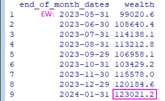
Der monatliche Durchschnitt des Gesamtvermögens lag bei rund USD113.145 von Ende Juni 2023 bis Ende Januar 2024 mit Kauf am 31.5.2023 zu möglichst gleichen Teilen und in ganzen Aktien mit einem Gesamt-Start-Kapital von USD100.000 => USD99.021 ausgegeben am 31.5.2023;
das Kapital am 31.1.2024 lag bei USD123.021, was im Übrigen auch der Peak wealth im ganzen Zeitraum auf Monatsend-Basis war:
=> fast 1/4 Turnover in nicht mal einem Jahr ist also schon erhöht nach meinem Geschmack
Magnificent 7: möglicher Portfolio-Turnover
wer kam eigentlich auf die Idee mit den "Magnificent Seven"?--> es war Michael Hartnett, Bank of America's chief investment strategist, ab Mai 2023: https://www.npr.org/2023/12/13/1216457187/wall-street-magnif…
In May, a few months after OpenAI debuted its ChatGPT tool, Hartnett noticed investors were channeling their enthusiasm for artificial intelligence into a small basket of established tech companies.
Mittlerweile sind es aber nur noch die "Fab Five":
January 30, 2024
https://finance.yahoo.com/video/magnificent-seven-stocks-now…
--> Nvidia, Meta Platforms, Google, Microsoft und Amazon
=> nach geschätzt 8 Monaten sind also so gesehen zwei Plätze frei geworden in den Magnificent 7: damit komme ich auf einen Turnover (nicht annualisiert; ohne Dividenden; Close-Preise; keine Gebühren etc.) nach SEC-PTR (https://de.wikipedia.org/wiki/Portfolio_Turnover_Ratio) von 24.6% in einem gleichgewichteten Magnificent 7-Portfolio (EW) mit Kauf am 31.5.2023 und Halten bis zum 31.1.2024 mit zwei Verkäufen an diesem Tag: Apple und Tesla
=> das entspricht auch in Größenordnung 2 / 7 = ~28.6%
Der monatliche Durchschnitt des Gesamtvermögens lag bei rund USD113.145 von Ende Juni 2023 bis Ende Januar 2024 mit Kauf am 31.5.2023 zu möglichst gleichen Teilen und in ganzen Aktien mit einem Gesamt-Start-Kapital von USD100.000 => USD99.021 ausgegeben am 31.5.2023;
das Kapital am 31.1.2024 lag bei USD123.021, was im Übrigen auch der Peak wealth im ganzen Zeitraum auf Monatsend-Basis war:

=> fast 1/4 Turnover in nicht mal einem Jahr ist also schon erhöht nach meinem Geschmack
Antwort auf Beitrag Nr.: 75.216.818 von faultcode am 04.02.24 19:37:54
Man kann diesen aber auch minimieren, so wie oben z.B. behauptet:
For example, the long-only sample UMVE portfolio for the 30 Momentum/ Volatility dataset has an estimated Sharpe ratio of 1.04. It is noteworthy, however, that this portfolio outperforms all of the benchmarks at the 1% significance level, and it does so despite having an average turnover of only 8% per year. Thus prohibiting short sales is an effective strategy for sharply reducing turnover, and it allows the sample UMVE portfolios to maintain a significant performance advantage over the benchmarks.
Daraus noch eine ältere Statistik, was so typische Werte für einen Portfolio-Turnover sein können:
Griffin and Xu (2009) provide a useful perspective on this issue. They report that an annualized turnover in the neighborhood of 100% is not uncommon for actively-managed mutual funds and that the turnover for a meaningful portion of the hedge funds examined is between 100% and 200% per year. Moreover, they find that hedge funds often have turnover approaching 200% per year and that the turnover for a small share of the funds studied is over 200% per year.
"Optimizing the Performance of Sample Mean-Variance Efficient Portfolios" (2): Portfolio-Turnover
wobei man bei solchen Optimierungen mMn durchaus auf den Turnover achten muss. (ich bin kein Freund von hohem Turnover)Man kann diesen aber auch minimieren, so wie oben z.B. behauptet:
For example, the long-only sample UMVE portfolio for the 30 Momentum/ Volatility dataset has an estimated Sharpe ratio of 1.04. It is noteworthy, however, that this portfolio outperforms all of the benchmarks at the 1% significance level, and it does so despite having an average turnover of only 8% per year. Thus prohibiting short sales is an effective strategy for sharply reducing turnover, and it allows the sample UMVE portfolios to maintain a significant performance advantage over the benchmarks.
Daraus noch eine ältere Statistik, was so typische Werte für einen Portfolio-Turnover sein können:
Griffin and Xu (2009) provide a useful perspective on this issue. They report that an annualized turnover in the neighborhood of 100% is not uncommon for actively-managed mutual funds and that the turnover for a meaningful portion of the hedge funds examined is between 100% and 200% per year. Moreover, they find that hedge funds often have turnover approaching 200% per year and that the turnover for a small share of the funds studied is over 200% per year.
mean-variance efficient portfolios <=> sample mean-variance efficient portfolios; conditioning information
Früher oder später stößt man auf dieses Akronym "SMV". Das steht im Kontext von "MV" für "Sample MV" oder eben "Sample Mean-Variance" (efficient portfolios).Gemeint ist, daß die Schätzungen für den Mean vector (= Return vector) und die Covariance matrix der Asset returns (Renditen) aus Stichproben stammen, eben den Samples.
Insofern sind diese beiden MV-efficient Portfolios von mir oben zu den Magnificent 7, 2019 - 2023, auch "SMV's":
• GMVP (Global Minimum Variance portfolio)
• TG (Tangent portfolio, Maximum Sharpe ratio portfolio)
Das ist insofern von Bedeutung, da es eben auch heutzutage Methoden (*) gibt, die mit diesen Schätzungen unweigerlich verbundenen Schätzfehler abzumildern und damit die historisch schlechte Performance out-of-sample solcher Portfolios zu beheben, z.B.:
2012: "Optimizing the Performance of Sample Mean-Variance Efficient Portfolios", Chris Kirby, Barbara Ostdiek: https://papers.ssrn.com/sol3/papers.cfm?abstract_id=1821284
=>
4 Closing Remarks
Mean-variance portfolio optimization has recently come under fire for its ostensibly poor performance in out-of-sample applications.
...
Our investigation supports a sharply contrasting view of the out-of-sample performance of mean-variance optimization.
...
To address the optimization problem in a more comprehensive fashion, we expand the scope of the analysis to encompass the effects of estimation risk, specification errors, and transaction costs on portfolio performance, and we use an adaptive empirical procedure to select the values of the unknown parameters that appear in the expression for the plug-in weights.
...
The resulting sample UMVE portfolios have well-behaved weights, reasonable turnover, and substantially higher estimated Sharpe ratios and certainty-equivalent returns than common performance benchmarks such as the 1/N portfolio and S&P 500 index.
...
UMVE = unconditionally mean-variance efficient
"Unconditional" geht dabei auf "conditioning information" zurück, bzw. das Fehler von solcher: https://onlinelibrary.wiley.com/doi/abs/10.1111/0022-1082.00…: (+)
The unconditionally efficient portfolio is the one that maximizes the measured performance.
...
This information structure can occur in economic policy problems, labor markets and in other agency problems. (+ interest rates, dividend yields, credit spreads z.B.)
=> insofern sind meine MV-Portfolios oben genau genommen: "unconditionally, sample mean-variance efficient portfolios" mit short sales prohibited und fully invested
"Unconditional" kann man dabei auch als "less informed" übersetzen.
(*) das ist so ähnlich, wie ich das hier mal angewandt habe, aber eben mit nicht sehr spektakulärem Erfolg:
Zitat von faultcode: ... Das Experiment bestand darin, für die Kovarianz für 2019 bis 2023 (covariance matrix of excess returns, CMER) eine Gewichtung mit EWMA (exponentially weighted moving average) vorzunehmen. Ich habe das hier gefunden:
... We are considering a realistic real world multi-asset allocation problem with semi-annual rebalancing of the portfolio. At each rebalancing date the covariance matrix was estimated from the previous 180 observations of weekly returns using an EWMA estimator with a half-life of one year.
...
Ich stellte aber nun fest, daß das in meinem Fall (erstaunlicherweise) nur zu geringfügig anderen Gewichten bei META und TSLA führte (kein Rebalancing; half-life of one year => decay coefficient = 0.9972488; lambda = 0.33, tau = 1.00): ... Daher habe ich diese Idee auch wieder verworfen.
(+)
The use of rolling estimators is common in research on mean-variance portfolio selection. A number of studies, for example, construct plug-in estimates of the portfolio weights by using a fixed-width rolling data window to estimate the mean vector and covariance matrix of asset returns. (2)
This approach seeks to balance the benefits of increasing the sample size against the costs of including more distant observations that are less likely to reflect current market conditions. Although the use of a fixed-width window has some intuitive appeal, it is typically less efficient than methods that exploit the full historical sample of asset returns. The literature suggests that exponentially-weighted rolling estimators are preferred from an efficiency perspective (see, e.g., Foster and Nelson, 1996).
Trading Spotlight
Antwort auf Beitrag Nr.: 75.215.030 von faultcode am 03.02.24 23:41:30
<ich weiß nicht, ob diese Frage portfoliotheoretisch sinnvoll ist; das ist meine eigene Idee>
Zur Erinnerung aus Beitrag Nr. 66:
Der Korrelations-Plot mit den bisherigen Portfolio-Typen sieht so aus:
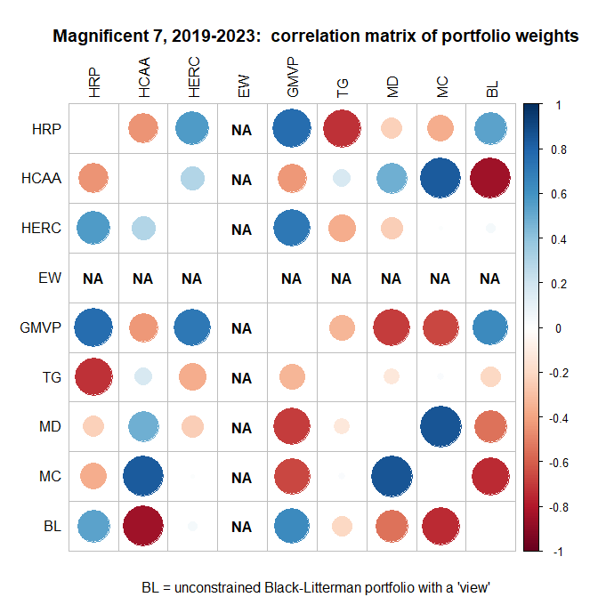
Korrelationskoeffizient (Pearson) = 1: "gleich"
Korrelationskoeffizient (Pearson) = -1: "gegenläufig"
EW (Equal Weight portfolio): hier ist die Standardabweichung der Portfoliogewichte (jeweils 1/7) 0.00 und damit hat man im Nenner des Korrelationskoeffizienten diese Null stehen => "NA", not available
=>
• die positivste Korrelation, wenn auch nicht "super-stark", ergibt sich zum GMVP (Global Minimum Variance portfolio) mit +63.3%
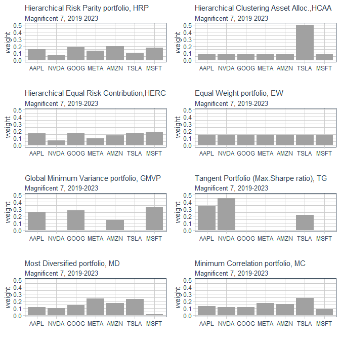
• die negativste Korrelation ergibt sich zum HCAA-Portfolio (Hierarchical Clustering Asset Allocation portfolio) mit -84.6%, was nicht verwunderlich ist, da im HCAA-Portfolio TSLA mit +50% gewichtet ist, siehe ganz oben rechts:
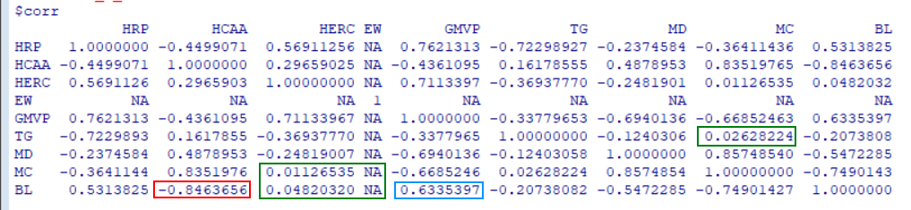
Interessant ist auch das HERC-Portfolio: es weist zwei Korrelationen nahe 0.0 auf, nämlich mit dem Minimum Correlation-Portfolio (MC) und eben meinem unbeschränkten Black-Litterman-Portfolio (BL).
Nebenbei: alle bisherigen Portfolio-Typen waren eindeutig, nur nicht das Black-Litterman-Portfolio, denn hier sind, je nach den Investor View's, eben unendlich viele Versionen vorstellbar (außer man ließe das Benchmark-Portfolio vom 29.12.2023 ohne Views gelten)
Magnificent 7, 2019 - 2023, mit BL (3): welches Portfolio ist am ähnlichsten?
Welches der bisherigen Portfolios ist meinem unbeschränkten Black-Litterman-Portfolio am nächsten, gemessen an der Korrelation der Portfolio-Gewichte?<ich weiß nicht, ob diese Frage portfoliotheoretisch sinnvoll ist; das ist meine eigene Idee>
Zur Erinnerung aus Beitrag Nr. 66:

Der Korrelations-Plot mit den bisherigen Portfolio-Typen sieht so aus:

Korrelationskoeffizient (Pearson) = 1: "gleich"
Korrelationskoeffizient (Pearson) = -1: "gegenläufig"
EW (Equal Weight portfolio): hier ist die Standardabweichung der Portfoliogewichte (jeweils 1/7) 0.00 und damit hat man im Nenner des Korrelationskoeffizienten diese Null stehen => "NA", not available
=>
• die positivste Korrelation, wenn auch nicht "super-stark", ergibt sich zum GMVP (Global Minimum Variance portfolio) mit +63.3%
• die negativste Korrelation ergibt sich zum HCAA-Portfolio (Hierarchical Clustering Asset Allocation portfolio) mit -84.6%, was nicht verwunderlich ist, da im HCAA-Portfolio TSLA mit +50% gewichtet ist, siehe ganz oben rechts:

Interessant ist auch das HERC-Portfolio: es weist zwei Korrelationen nahe 0.0 auf, nämlich mit dem Minimum Correlation-Portfolio (MC) und eben meinem unbeschränkten Black-Litterman-Portfolio (BL).
Nebenbei: alle bisherigen Portfolio-Typen waren eindeutig, nur nicht das Black-Litterman-Portfolio, denn hier sind, je nach den Investor View's, eben unendlich viele Versionen vorstellbar (außer man ließe das Benchmark-Portfolio vom 29.12.2023 ohne Views gelten)
Antwort auf Beitrag Nr.: 75.214.745 von faultcode am 03.02.24 21:39:47

..und im Vergleich zum nach Marktkapitalisierung gewichteten Benchmark-Portfolio vom 29.12.2023 so:
Nachdem alle bisherigen Portfolios keine Leerverkäufe vorsehen und voll investiert sind, habe ich TSLA auf Gewicht 0 gesetzt und ohne weitere Optimierungen die anderen 6 Portfolio-Komponenten einfach proportional hochskaliert mit Summe 1.00 wieder:
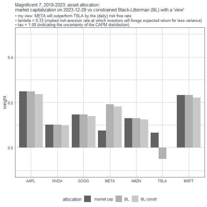
constr = constrained
Magnificent 7, 2019 - 2023, mit BL (2): das unbeschränkte und beschränkte BL-Portfolio
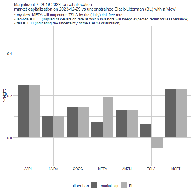
die oben errechneten Portfolio-Gewichte sehen so aus:
..und im Vergleich zum nach Marktkapitalisierung gewichteten Benchmark-Portfolio vom 29.12.2023 so:

Nachdem alle bisherigen Portfolios keine Leerverkäufe vorsehen und voll investiert sind, habe ich TSLA auf Gewicht 0 gesetzt und ohne weitere Optimierungen die anderen 6 Portfolio-Komponenten einfach proportional hochskaliert mit Summe 1.00 wieder:

constr = constrained
Antwort auf Beitrag Nr.: 75.214.892 von faultcode am 03.02.24 22:41:15
ein Wort noch zu meiner View, Design, Link, Linking oder Pick matrix P (K x N) von oben, die meine willkürliche Wahl eines "Investor View's" auf die Magnificent 7 ist:
P <- structure(c(0, 0, 0, 1, 0, -1, 0), .Dim = c(1L, 7L), .Dimnames = list(c("View 1"), tckr))
=>
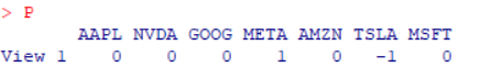
=> in meinem "Vector of confidences" habe ich einen "relative view" mit Summe 0 = +1 -1 eingenommen und damit auch nur einen solchen Vektor. Ich hätte da noch mehr Views einnehmen können, z.B.:
NVDA wird weiterhin super laufen:
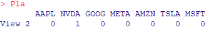
=> das wäre dann ein "absolute view" gewesen. Siehe z.B.:
2023: Portfolio Optimization: The Black-Litterman Allocation Method
https://wire.insiderfinance.io/portfolio-optimization-the-bl… --> Views:
...
Absolute views have a single 1 in the column corresponding to the asset’s order in the asset universe, while relative views have a positive number in the outperforming asset column, and a negative number in the underperforming asset column. Each row for relative views in P must sum up to 0, ...
Der Fantasie sind da keine Grenzen gesetzt und damit auch nicht den erwarteten Renditen (expected returns) im korrespondierenden K x 1 Column Vector Q.
Im R-Code-Beispiel aus oben (https://rpubs.com/rvanzini/BLR) sieht die View matrix mit 4 ETF's und 3 Views (2 x relativ, 1 x absolut) z.B. so aus:
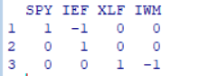
Ich glaube, an keiner Stelle des klassischen Black-Litterman-Modell's wurde nach 1992 soviel geschraubt und erweitert wie bei den Investor Views.
Magnificent 7, 2019 - 2023, mit BL (1c): View matrix P
(2)ein Wort noch zu meiner View, Design, Link, Linking oder Pick matrix P (K x N) von oben, die meine willkürliche Wahl eines "Investor View's" auf die Magnificent 7 ist:
P <- structure(c(0, 0, 0, 1, 0, -1, 0), .Dim = c(1L, 7L), .Dimnames = list(c("View 1"), tckr))
=>

=> in meinem "Vector of confidences" habe ich einen "relative view" mit Summe 0 = +1 -1 eingenommen und damit auch nur einen solchen Vektor. Ich hätte da noch mehr Views einnehmen können, z.B.:
NVDA wird weiterhin super laufen:

=> das wäre dann ein "absolute view" gewesen. Siehe z.B.:
2023: Portfolio Optimization: The Black-Litterman Allocation Method
https://wire.insiderfinance.io/portfolio-optimization-the-bl… --> Views:
...
Absolute views have a single 1 in the column corresponding to the asset’s order in the asset universe, while relative views have a positive number in the outperforming asset column, and a negative number in the underperforming asset column. Each row for relative views in P must sum up to 0, ...
Der Fantasie sind da keine Grenzen gesetzt und damit auch nicht den erwarteten Renditen (expected returns) im korrespondierenden K x 1 Column Vector Q.
Im R-Code-Beispiel aus oben (https://rpubs.com/rvanzini/BLR) sieht die View matrix mit 4 ETF's und 3 Views (2 x relativ, 1 x absolut) z.B. so aus:

Ich glaube, an keiner Stelle des klassischen Black-Litterman-Modell's wurde nach 1992 soviel geschraubt und erweitert wie bei den Investor Views.
Antwort auf Beitrag Nr.: 75.214.745 von faultcode am 03.02.24 21:39:47
(1) das mit einer italienischen Quelle ist möglicherweise kein Zufall. Früher oder später stößt man nämlich vielleicht auf diese Quelle:
2010: "The Black-Litterman Approach: Original Model and Extensions", von Attilio Meucci: https://papers.ssrn.com/sol3/papers.cfm?abstract_id=1117574
welches in kürzerer Form hier erschien: https://onlinelibrary.wiley.com/doi/book/10.1002/97804700616…
Attilio Meucci hat noch mehr Papiere zum Thema Black-Litterman verfasst: https://papers.ssrn.com/sol3/cf_dev/AbsByAuth.cfm?per_id=403…, zu nennen vielleicht "Fully Flexible Views: Theory and Practice" von 2010: https://papers.ssrn.com/sol3/papers.cfm?abstract_id=1213325
...und gleich ein ganzes und mMn sehr schönes, allgemein ausgerichtetes Buch zum Thema "Risk and Asset Allocation" verfasst: https://link.springer.com/book/10.1007/978-3-540-27904-4
Von 2005 ist es natürlich nicht mehr der letzte Schrei, auch nicht von ihm selber zu BL, aber manchmal reichen die Basics auch schon, vor allem noch aus einer Zeit bevor Quantitative finance durch die undurchsichtige "Deep learning-Soße" gezogen wurde. Black-Litterman ist natürlich auch drin:
https://en.wikipedia.org/wiki/Attilio_Meucci: seit 2010 betreibt er eine "e-learning platform for quantitative finance": https://www.arpm.co/
Magnificent 7, 2019 - 2023, mit BL (1b): Attilio Meucci
Zwei Bemerkungen noch zu diesem R-code:(1) das mit einer italienischen Quelle ist möglicherweise kein Zufall. Früher oder später stößt man nämlich vielleicht auf diese Quelle:
2010: "The Black-Litterman Approach: Original Model and Extensions", von Attilio Meucci: https://papers.ssrn.com/sol3/papers.cfm?abstract_id=1117574
welches in kürzerer Form hier erschien: https://onlinelibrary.wiley.com/doi/book/10.1002/97804700616…
Attilio Meucci hat noch mehr Papiere zum Thema Black-Litterman verfasst: https://papers.ssrn.com/sol3/cf_dev/AbsByAuth.cfm?per_id=403…, zu nennen vielleicht "Fully Flexible Views: Theory and Practice" von 2010: https://papers.ssrn.com/sol3/papers.cfm?abstract_id=1213325
...und gleich ein ganzes und mMn sehr schönes, allgemein ausgerichtetes Buch zum Thema "Risk and Asset Allocation" verfasst: https://link.springer.com/book/10.1007/978-3-540-27904-4
Von 2005 ist es natürlich nicht mehr der letzte Schrei, auch nicht von ihm selber zu BL, aber manchmal reichen die Basics auch schon, vor allem noch aus einer Zeit bevor Quantitative finance durch die undurchsichtige "Deep learning-Soße" gezogen wurde. Black-Litterman ist natürlich auch drin:

https://en.wikipedia.org/wiki/Attilio_Meucci: seit 2010 betreibt er eine "e-learning platform for quantitative finance": https://www.arpm.co/
Antwort auf Beitrag Nr.: 75.213.437 von faultcode am 03.02.24 13:21:32
S_cov_var <- as.matrix(stats::cov(as.matrix(dat_assets_daily_returns_log_exc3)))
#
tckr <- c('AAPL', 'NVDA', 'GOOG', 'META', 'AMZN', 'TSLA', 'MSFT')
lambda <- 0.33 # (0.08 - 0.05) / (0.3000^2) = 0.33
P <- structure(c(0, 0, 0, 1, 0, -1, 0), .Dim = c(1L, 7L), .Dimnames = list(c("View 1"), tckr))
Q <- 7.79124e-05 # daily interest log return from 2019 to 2023
tau <- 1.0 # see: Erindi Allaj, 2017: "The Black-Litterman Model, A Consistent Estimation of the Parameter Tau"
Omega <- P %*% S_cov_var %*% t(P) * tau
first_BL <- solve(solve(tau * S_cov_var) + t(P) %*% solve(Omega) %*% P) # solve(x) = x^(-1)
# Magnificient 7, market caps on 2023-12-29:
w <- c(0.24873307, 0.10160339, 0.14580045, 0.07560023, 0.13043117, 0.06563097, 0.23220071)
PI <- lambda * S_cov_var %*% w
second_BL <- solve(tau * S_cov_var) %*% PI + t(P) %*% solve(Omega) %*% Q
ER_BL <- first_BL %*% second_BL
Var_BL <- S_cov_var + solve(solve(tau * S_cov_var) + t(P) %*% solve(Omega) %*% P)
BL_weights_vector <- solve(lambda * Var_BL) %*% ER_BL
BL_weights_vector <- BL_weights_vector / sum(BL_weights_vector)
print(sum(BL_weights_vector)) # only a check for 1.00
#
# nice printing of the final, unconstrained BL weights:
arggs <- list(digits = 2, nsmall = 3)
caption1 = paste("lambda:", lambda, ",", "tau:", round(tau, digits = 7))
knitr::kable(tibble(asset = tckr,
w_BL = BL_weights_vector,
w_PI = w,
diff = w_BL - w_PI),
format.args = arggs,
caption = caption1
)
Die täglichen Überrenditen (dat_assets_daily_returns_log_exc3), also die E(r) - rf von oben, und der tägliche, risikolose Zinssatz (Q), beide in logarithmisierter Form, habe ich schon zuvor an anderer Stelle berechnet; die Portfolio-Gewichte nach Marktkapitalisierung für den 29.12.2023, w_PI ("market portfolio", "benchmark portfolio"), auch.
Wenn dann alles OK ist, sollte am Ende dieser Gewichtsvektor w_BL mit meinem "View" für mein Black-Litterman-Portfolio mit den Magnificent 7 ab dem 2.1.2024 herauskommen:
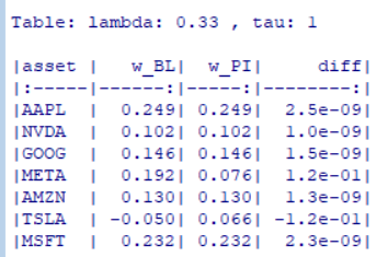
Und da dieses Portfolio unbeschränkt ist, eben mit 5% Leerverkaufsquote für TSLA und damit folglich mit erhöht positivem Gewicht für META. In Summe sollte der Gesamt-Gewichtsvektor sinnigerweise 1.00 ergeben.
Eine wichtige Inspirationsquelle war dieser R-Code mit Beschreibung in italienischer Sprache: "Applicazioni del modello di Black-Litterman in R" : https://rpubs.com/rvanzini/BLR
Dort findet man noch mehr um obigen "Core code" herum und wie man die Ergebnisse visualisieren kann.
Man muss mMn nämlich echt aufpassen, was man so im Netz an Computer-Code, egal ob in R oder nicht, zu Black-Litterman vorfindet.
Magnificent 7, 2019 - 2023, mit BL (1a): R-code (minimal)
# covariance matrix, 2019-2023:S_cov_var <- as.matrix(stats::cov(as.matrix(dat_assets_daily_returns_log_exc3)))
#
tckr <- c('AAPL', 'NVDA', 'GOOG', 'META', 'AMZN', 'TSLA', 'MSFT')
lambda <- 0.33 # (0.08 - 0.05) / (0.3000^2) = 0.33
P <- structure(c(0, 0, 0, 1, 0, -1, 0), .Dim = c(1L, 7L), .Dimnames = list(c("View 1"), tckr))
Q <- 7.79124e-05 # daily interest log return from 2019 to 2023
tau <- 1.0 # see: Erindi Allaj, 2017: "The Black-Litterman Model, A Consistent Estimation of the Parameter Tau"
Omega <- P %*% S_cov_var %*% t(P) * tau
first_BL <- solve(solve(tau * S_cov_var) + t(P) %*% solve(Omega) %*% P) # solve(x) = x^(-1)
# Magnificient 7, market caps on 2023-12-29:
w <- c(0.24873307, 0.10160339, 0.14580045, 0.07560023, 0.13043117, 0.06563097, 0.23220071)
PI <- lambda * S_cov_var %*% w
second_BL <- solve(tau * S_cov_var) %*% PI + t(P) %*% solve(Omega) %*% Q
ER_BL <- first_BL %*% second_BL
Var_BL <- S_cov_var + solve(solve(tau * S_cov_var) + t(P) %*% solve(Omega) %*% P)
BL_weights_vector <- solve(lambda * Var_BL) %*% ER_BL
BL_weights_vector <- BL_weights_vector / sum(BL_weights_vector)
print(sum(BL_weights_vector)) # only a check for 1.00
#
# nice printing of the final, unconstrained BL weights:
arggs <- list(digits = 2, nsmall = 3)
caption1 = paste("lambda:", lambda, ",", "tau:", round(tau, digits = 7))
knitr::kable(tibble(asset = tckr,
w_BL = BL_weights_vector,
w_PI = w,
diff = w_BL - w_PI),
format.args = arggs,
caption = caption1
)
Die täglichen Überrenditen (dat_assets_daily_returns_log_exc3), also die E(r) - rf von oben, und der tägliche, risikolose Zinssatz (Q), beide in logarithmisierter Form, habe ich schon zuvor an anderer Stelle berechnet; die Portfolio-Gewichte nach Marktkapitalisierung für den 29.12.2023, w_PI ("market portfolio", "benchmark portfolio"), auch.
Wenn dann alles OK ist, sollte am Ende dieser Gewichtsvektor w_BL mit meinem "View" für mein Black-Litterman-Portfolio mit den Magnificent 7 ab dem 2.1.2024 herauskommen:

Und da dieses Portfolio unbeschränkt ist, eben mit 5% Leerverkaufsquote für TSLA und damit folglich mit erhöht positivem Gewicht für META. In Summe sollte der Gesamt-Gewichtsvektor sinnigerweise 1.00 ergeben.
Eine wichtige Inspirationsquelle war dieser R-Code mit Beschreibung in italienischer Sprache: "Applicazioni del modello di Black-Litterman in R"
 : https://rpubs.com/rvanzini/BLR
Dort findet man noch mehr um obigen "Core code" herum und wie man die Ergebnisse visualisieren kann.
Man muss mMn nämlich echt aufpassen, was man so im Netz an Computer-Code, egal ob in R oder nicht, zu Black-Litterman vorfindet.


